荧光显微镜的共定位分析及绘图的Python脚本(含代码下载链接)
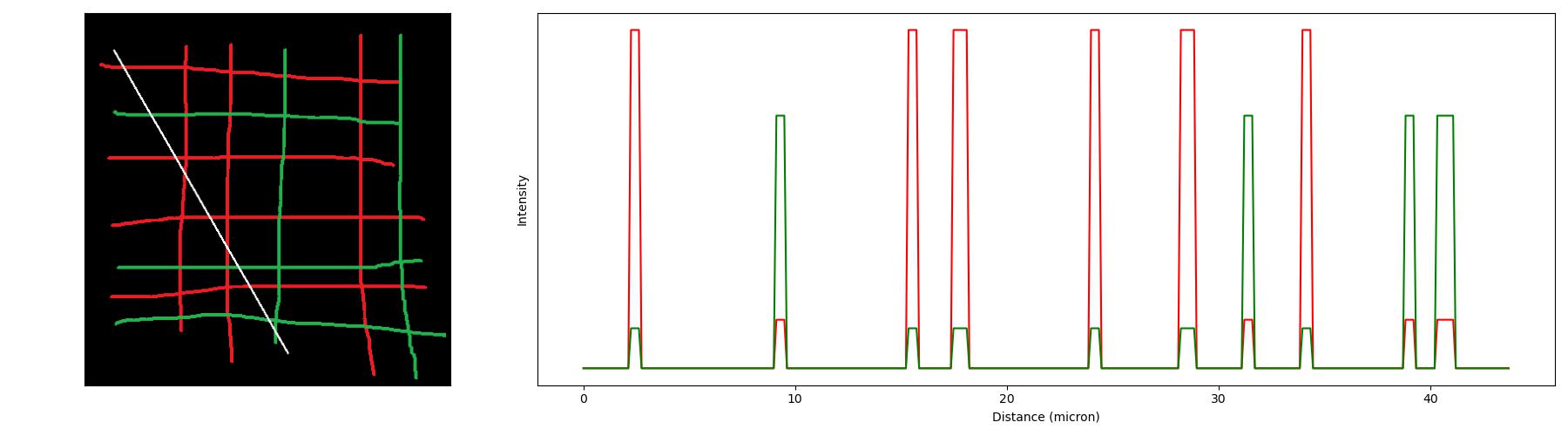
共定位是荧光图像能够得到的最最基础的信息,其可以作为分子互作的弱证据,分子在特定结构富集的强证据。该分析的常见操作是使用ImageJ的
line profile功能,但在imageJ中完成时,无法很好地绘制出好看的图,并准确输出划线的位置。本脚本是基于Python的,给实验室做共定位分析绘图用的,可以直接使用命令行调用,自动排图并计算皮尔逊相关系数
脚本实现的基思路
使用opencv读取图像、识别鼠标事件、绘制扫描线,使用argparse制作命令行工具,自己写函数读取线上的全部数值,使用matplotlib绘图并保存输出图像
脚本下载
drawCoLoc.py
import cv2
import argparse
import datetime
import numpy as np
from matplotlib import gridspec
from matplotlib import pyplot as plt

btn_down = False
SCALE = 9.2661  # pixel per micron
RED = 'mcherry'
GREEN = 'GFP'
BLUE = 'DAPI'

parser = argparse.ArgumentParser(usage="drawCoLoc -f RGB_image_file_path [<-b> <--noPCC> <-n> <-r resolution>]",
                                 description="\n\nHere's a script for co-localization analysis (line profile) on RGB image")
parser.add_argument('-f', metavar='file path', help='the path of the RGB image', dest="fpath", type=str, required=True)
parser.add_argument('-b', '--blue', help='add this parameter if you need blue channel', default=False, action='store_true')
parser.add_argument('--noPCC', help='add this parameter if you do not need label Person Cor', default=False, action='store_true')
parser.add_argument('-n', '--normalization', help='add this parameter if you need normalization for each channel', default=False, action='store_true')
parser.add_argument('-r', help='resolution if you need modify default values 9.2661 for dv usual use', dest='resolution', type=float, default=SCALE)

def get_points(im):
    # Set up data to send to mouse handler
    data = {}
    data['im'] = im.copy()
    data['lines'] = []
    # Set the callback function for any mouse event
    cv2.imshow("Image", im)
    cv2.setMouseCallback("Image", mouse_handler, data)
    cv2.waitKey(0)
    # Convert array to np.array in shape n,2,2
    points = np.uint16(data['lines'])
    draw_coloc(im, data['im'], points)
    # return points, data['im']
    return True


def mouse_handler(event, x, y, flags, data):
    global btn_down
    if event == cv2.EVENT_LBUTTONUP and btn_down:
        # if you release the button, finish the line
        btn_down = False
        data['lines'][0].append((x, y))
        cv2.line(data['im'], data['lines'][0][0], data['lines'][0][1], (255, 255, 255), 2)
        cv2.imshow("Image", data['im'])

    elif event == cv2.EVENT_MOUSEMOVE and btn_down:
        # thi is just for a ine visualization
        image = data['im'].copy()
        cv2.line(image, data['lines'][0][0], (x, y), (255, 255, 255), 1)
        cv2.imshow("Image", image)

    elif event == cv2.EVENT_LBUTTONDOWN and len(data['lines']) < 2:
        btn_down = True
        data['lines'].insert(0, [(x, y)])  # prepend the point
        cv2.imshow("Image", data['im'])


def normalization(x):
    _range = np.max(x) - np.min(x)
    return (x - np.min(x)) / _range


def get_line(img, pts):
    c = []
    for p in pts:
        dx, dy = int(p[-1, 0]) - int(p[0, 0]), int(p[-1, 1]) - int(p[0, 1])
        if dx >= dy:
            k, d = dy / dx, ((dx * dx + dy * dy) ** (1 / 2)) / args.resolution
            for t in range(dx):
                i = int(p[0, 0]) + t
                j = int(p[0, 1]) + round(k * t)
                c.append(img[j, i, ::-1])
            ds = np.linspace(0, d, dx)
            c = np.array(c).T
        else:
            k, d = dx / dy, ((dx * dx + dy * dy) ** (1 / 2)) / args.resolution
            for t in range(dy):
                i = int(p[0, 0]) + round(k * t)
                j = int(p[0, 1]) + t
                c.append(img[j, i, ::-1])
            ds = np.linspace(0, d, dy)
            c = np.array(c).T
    if args.normalization:
        c = [normalization(x) for x in c]
    return ds, c


def draw_coloc(img, final_image, pts):
    ds, c = get_line(img, pts)
    cor = np.corrcoef(c[0], c[1])
    fig = plt.figure(figsize=(18, 5))
    gs = gridspec.GridSpec(1, 2, width_ratios=[1, 2])
    ax0 = plt.subplot(gs[0])
    ax0.imshow(final_image[:, :, ::-1]);
    ax0.set_xticks([]);
    ax0.set_yticks([])
    ax1 = plt.subplot(gs[1])
    ax1.plot(ds, c[0], color='red', label=RED)
    ax1.plot(ds, c[1], color='green', label=GREEN)
    if args.blue:
        ax1.plot(ds, c[2], color='blue', label=BLUE)

    if args.noPCC:
        print(f"Person's corr={cor[0][1]:.2f}")
    else:
        ax1.text(0.85, 0.92, f"Person's corr={cor[0][1]:.2f}", fontsize=12, transform=ax1.transAxes)
    # plt.legend(loc='lower center')

    ax1.set_ylabel('Intensity');
    ax1.set_yticks([])
    ax1.set_xlabel('Distance (micron)')
    dt = datetime.datetime.now().strftime('%Y%m%d %H%M%S')
    plt.tight_layout()
    plt.savefig(f'.\\{"".join(args.fpath.split(".")[:-1])}-{dt}.jpg')
    plt.show()


if __name__ == '__main__':
    args = parser.parse_args()
    img = cv2.imread(args.fpath, 1)
    if get_points(img):
        print('Succeed!')
脚本的使用方法
在安装Python环境后,按照如下提示输入脚本的命令行即可调用。调用会弹出图像窗口,用鼠标划线后按任意键即可自动生成共定位分析图像,并保存在与原图像相同的文件夹下。
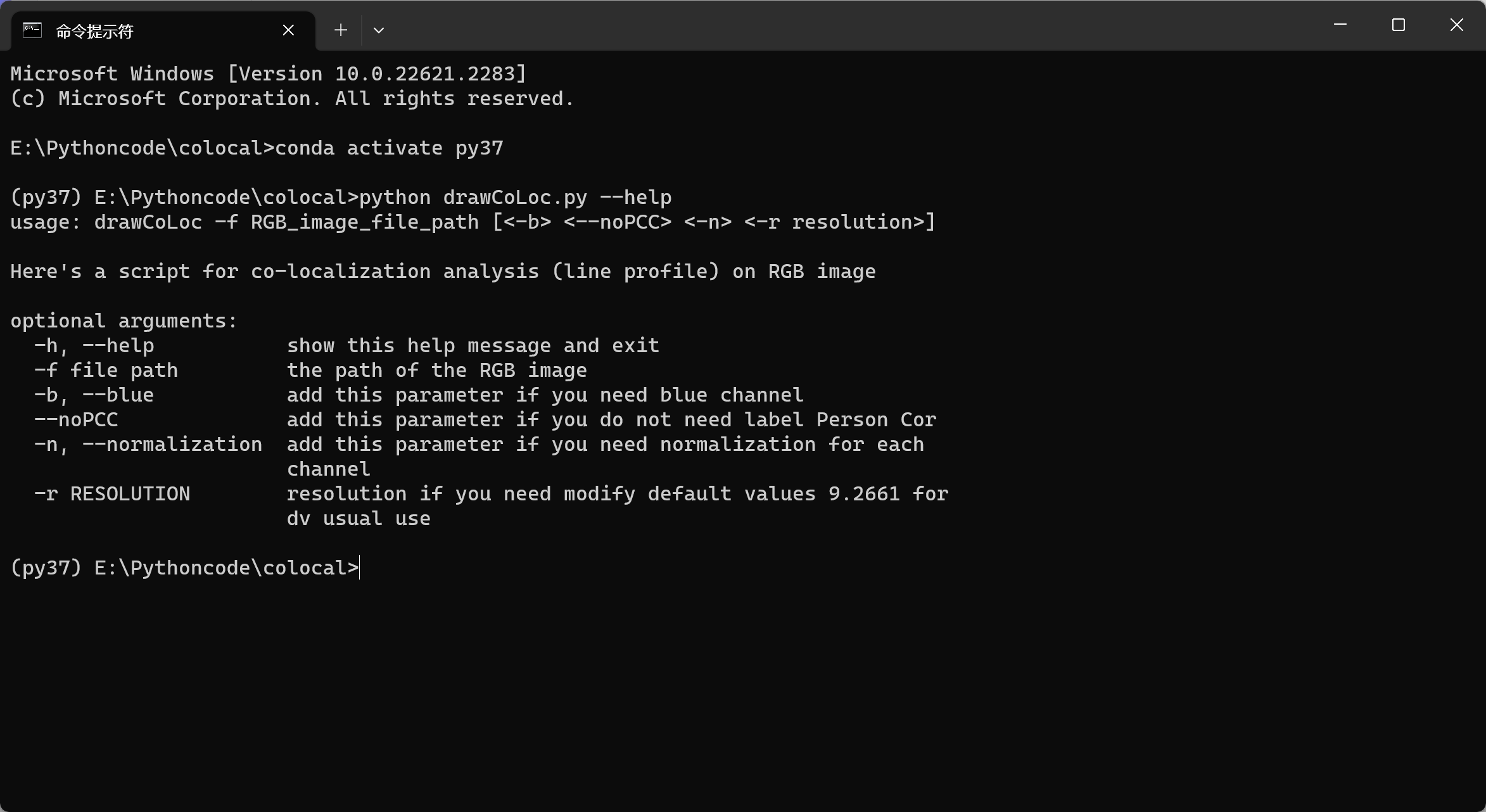
python drawCoLoc.py -f ./1.png --noPCC